01 Introduction

This tutorial covers the basics of working with raster and vector spatial data within QGIS. After completing this tutorial you will learn how to load datasets into a new QGIS project; manipulate layer symbology based on attribute information; and use the print composer to compose and export maps from QGIS.

Deliverables

One map of trees in NYC composed as a 8.5x11 page (landscape or portrait orientation) exported as a PDF. Your map must include standard map elements outlined in the layout portion of this tutorial.

File management

All datasets within your QGIS project are not embedded but rather are stored as links to wherever the dataset is stored. Because of this file and data management is an important component of work in QGIS.

Create a new folder for your work on tutorials for this course. Inside it create a data folder and then and original and a processed folder. All downloaded datasets should be saved in the data>original folder. Any new datasets you create in the process of completing the modules should be saved within the data>processed folder.

Data

In this tutorial you will be making a series of maps about the urban forest in New York City. Download the following datasets:

• New York City Landcover 2010 (3ft version). A raster dataset created to describe major land use categories for New York City derived from satellite imagery. Full metadata and other downloads available via NYC Open Data [here] Download this dataset (Land Cover 2010.zip) and unzip its contents. You should have a folder titled Land_Cover_2010 with five files in it. Also from the above page download the Data Dictionary for this dataset: Landcover2010_DataDictionary_20171012.xlsx. Save it within the Land_Cover_2010 folder.
• New York City 2015 Street Tree Census. (Download from Files>Data on the class courseworks website.) This dataset was collected by more than 2000 volunteers visiting each street tree within the five boroughs of NYC. For more background on this amazing effort (the third such census over the past 30 years) see the NYC Parks department website here. The link above provides a subset of the data for an area in Harlem to make for easier processing. For those interested the full dataset is available for download directly via NYC Open Data here

QGIS interface

Open QGIS and create a new project.

QGIS interface

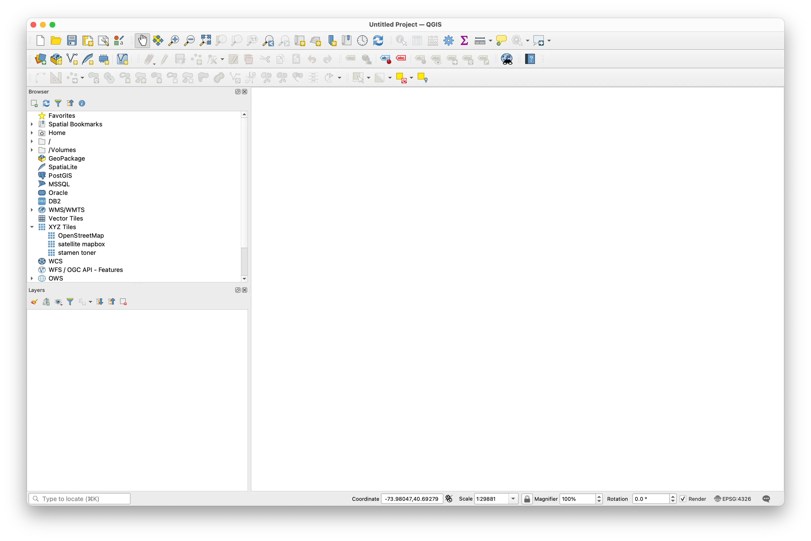
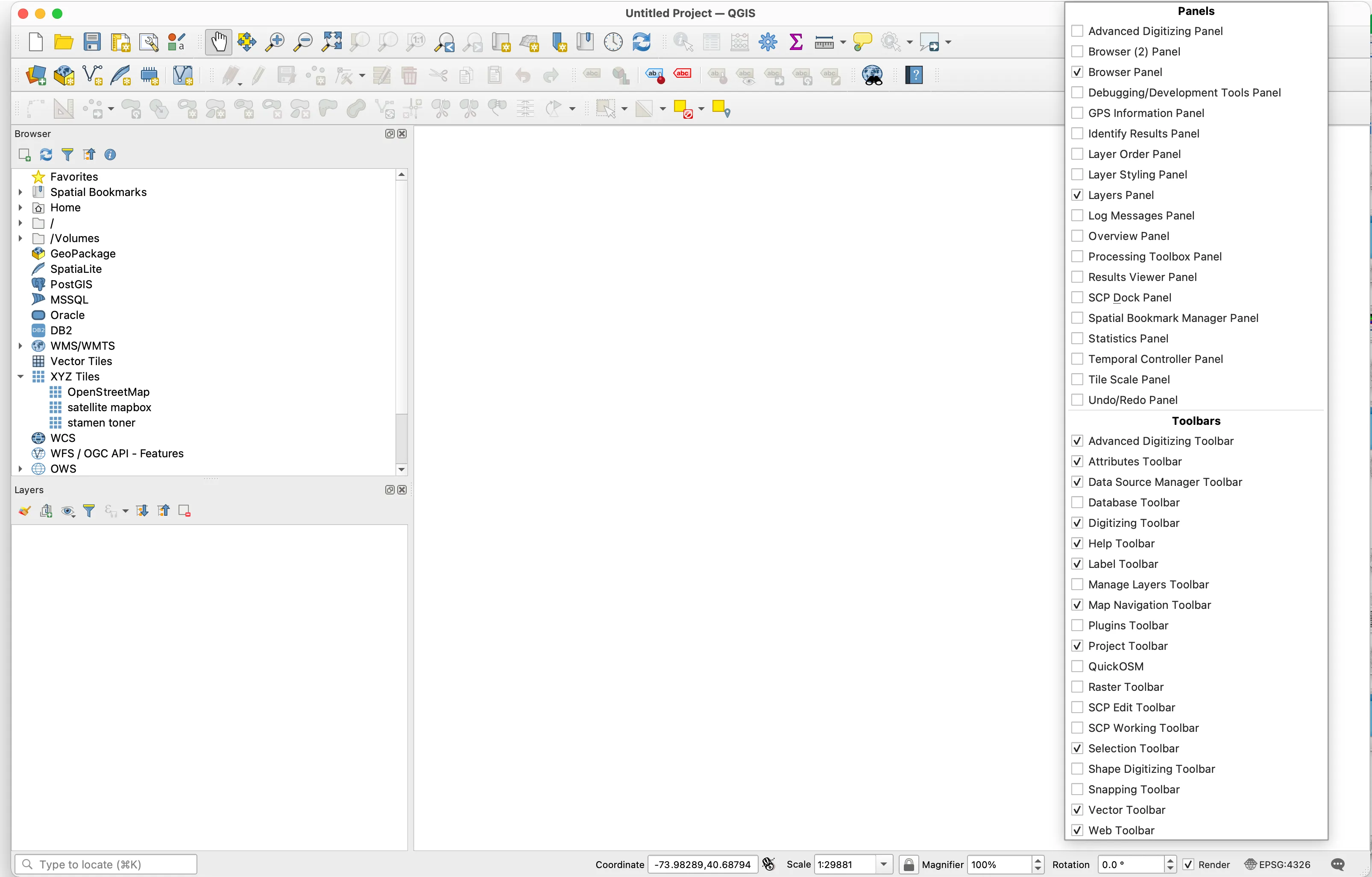
The QGIS interface consists of a selection of Panels and Toolbars and a Map canvas.

All toolbars and panels can be moved or removed from the QGIS interface. If you need to access a specific panel or toolbar right click anywhere within the grey areas surrounding a panel or toolbar to open the toolbar and panels browser (shown at right).

The Browser Panel provides the ability to browse, search and inspect spatial datasets from your local file system, database connections, and online sources.

The Layers Panel will show all datasets (layers) that you have added to your project. After adding datasets to your project you can access properties and analytic tools for each layer via its name in the layer panel. The order of the datasets listed here controls their rendering order in the **Map canvas`.

The Map canvas provides a view of the datasets you have added to your project.

Toolbars provide access to various tools within the program.

Exercise

Adding raster data: mapping tree cover from land use

The first layer we will add to our project is a raster dataset of landcover for New York City from 2010. This dataset was developed by researchers using satellite imagery to identify major categories of materials (cement, buildings, open ground, water, vegetation, tree cover) for all of New York City.

We will use this layer to visualize the canopy of New York City’s trees.

From the top menu bar select Layer and then Add Layer > Add Raster Layer.

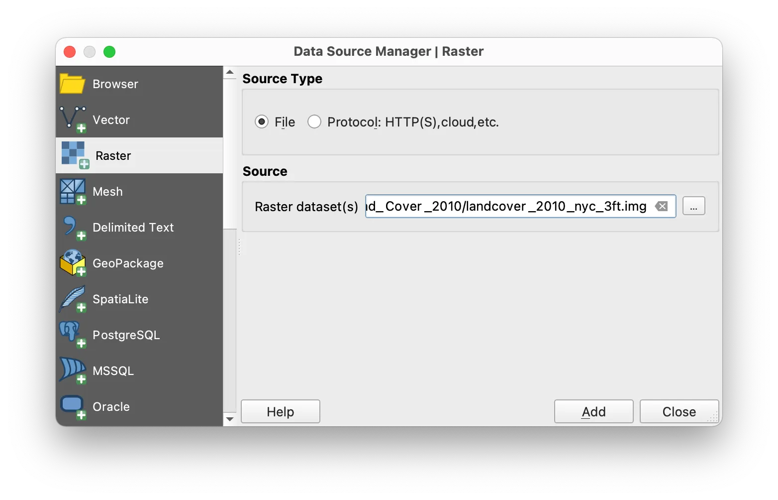
Data source manager

When the Data Source Manager menu appears select the Source Type as File then click on the ... and navigate to the Land_cover_2010 folder within data folder you created for this series of modules. Select the file named landcover_2010_nyc_3ft.img. Take care to select the file with the .img file extension. The five files with the same name except for their file extension together comprise this particular raster dataset (for more on the specific file format that this dataset uses see here). QGIS will do the work of interpreting each of the five files together. Click Add. Then click Close.

The land cover dataset’s name should now appear in the layers panel and the dataset should be visible in the map canvas.

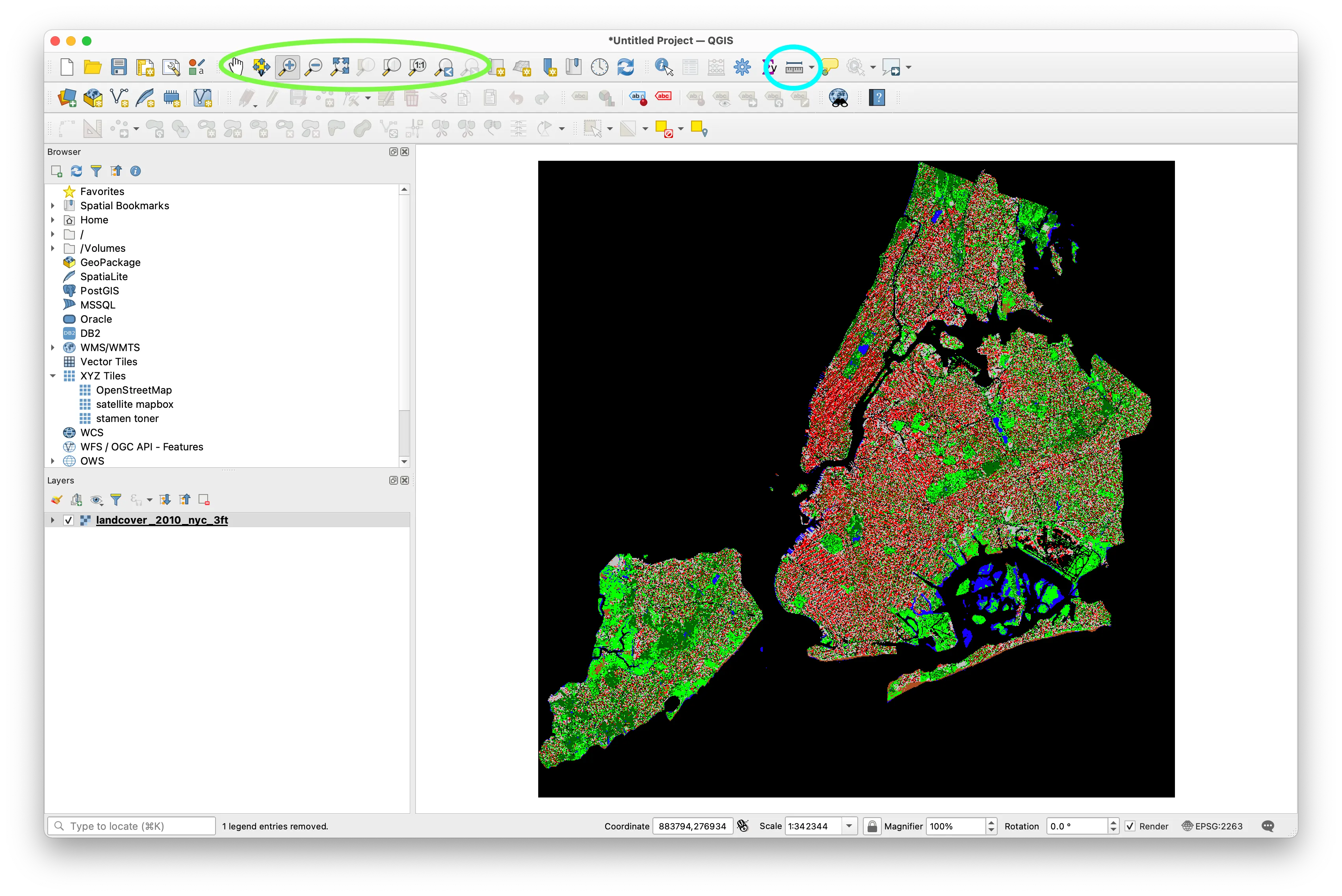Land cover data for New York City

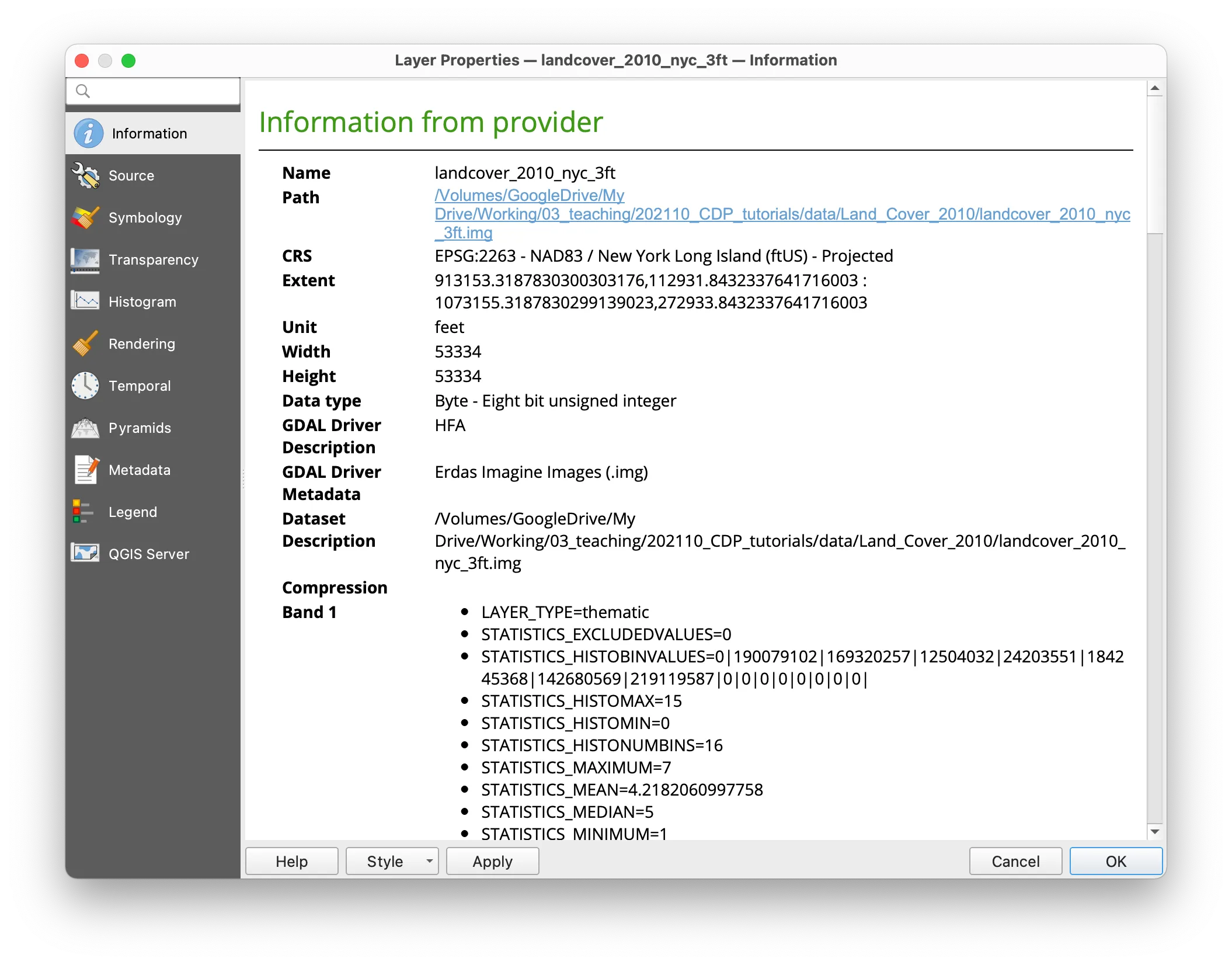
Open the Layer Properties menu for this dataset to look at its source and coordinate reference system information. This is always a good thing to do when you add a new dataset to your project.

Notice that the coordinate reference system is already defined as EPSG:2263 which refers to the New York State Plane Coordinate reference system for the Long Island region. This is the projected coordinate reference system that produces the smallest level of distortion for NYC and should be used for all local maps of NYC. Because the dataset already uses this coordinate reference system

Layer Properties panel 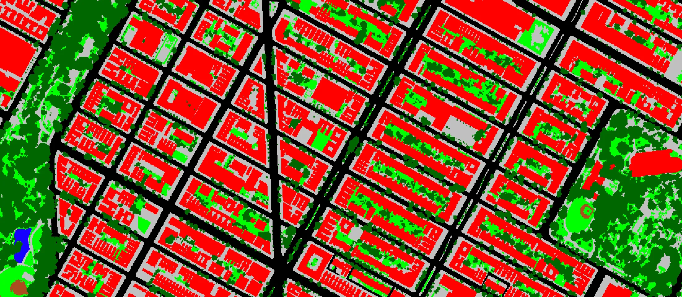A closeup of land cover data for NYC

Save your project within the folder you created for this series of modules. Save the QGIS project as a .qgz file.

Use the map navigation tools (circled above in green) to zoom to an area that interests you. The view on the right shows Harlem between Morningside and Marcus Garvey parks.

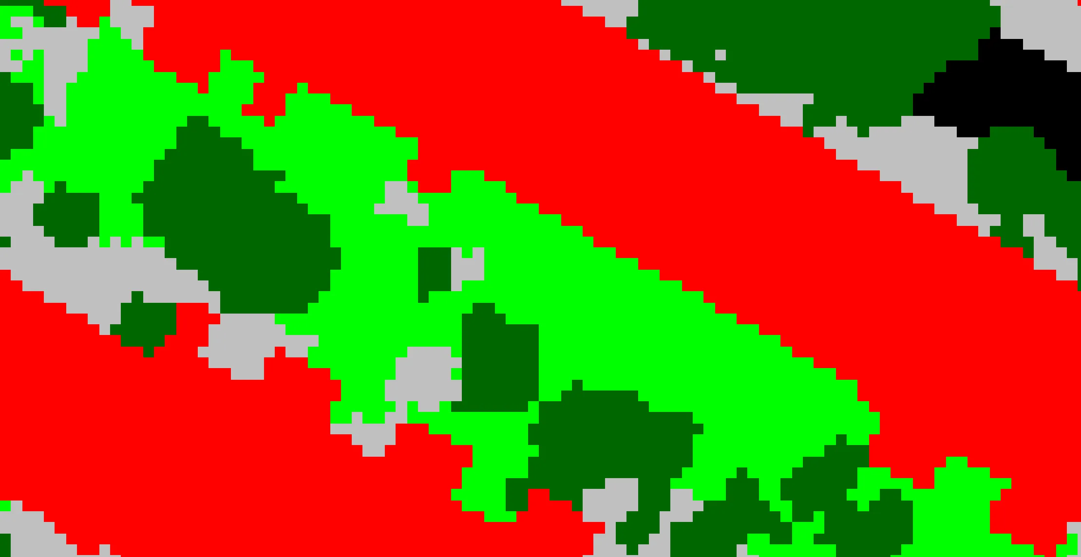Individual raster cells visible in NYC land cover data

Continue to zoom in until individual raster cells are visible.

Next use the Measure Line tool (circled above in cyan) to measure the size of each raster cell (aka pixel). Set the units to feet, in the map canvas click where you want to start measuring then click again where you want to stop. Each cell is 3 feet. This matches the information conveyed in the metadata for the dataset.

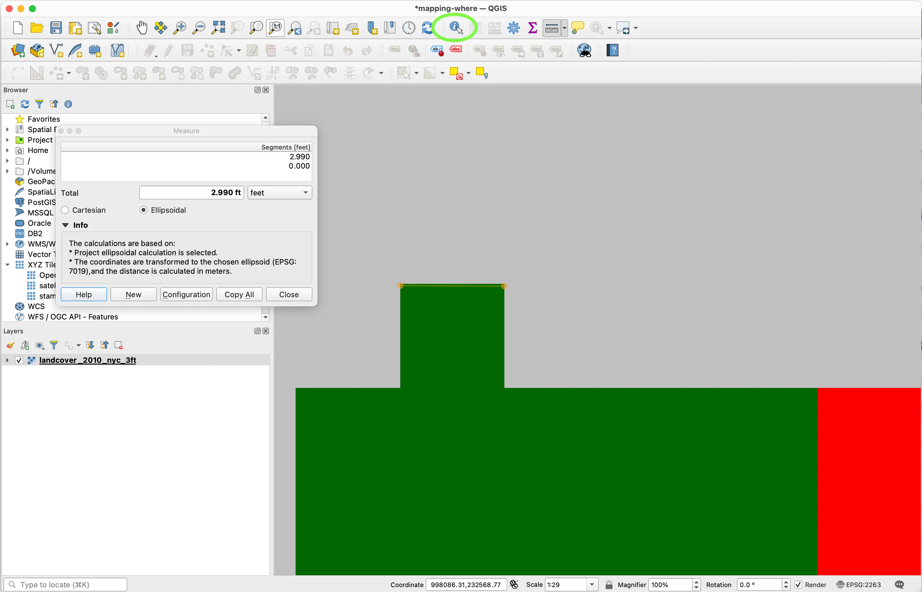The measuring tool

Next use the identify features tool (circled in green above) to examine the value contained in a few of the rasters cells. Remember for raster datasets each cell represents a specific area on the earths surface (its cell size) and each cell has exactly one numeric value. With the identify features tool selected click on a raster cell. The Identify Results Panel will show you the numeric value for each cell that you click.

The meaning of these values is explained in the data dictionary provided with the data (see Landcover2010_DataDictionary_20171012.xlsx within the Land_Cover_2010 folder). Open this file from your data folder to take a look at it. Notice that cells with a value of 1 correspond to areas classified as within the ‘tree canopy’ for NYC.

Our goal in this part of the module is to design a map showing the tree canopy for New York City.

To do this we will manipulate the symbology for this land cover layer. Right click on the layer’s name in the layers panel. Open the layer Properties menu. Open the Symbology tab. Currently you’ll notice that each numeric value, which each correspond to a specific land cover designation, has been assigned a unique color. You can change the color assigned to each land cover category by right clicking on a row in the symbology menu and then selecting Change Color.

Select all of the values except for 1. Right click to change their color.

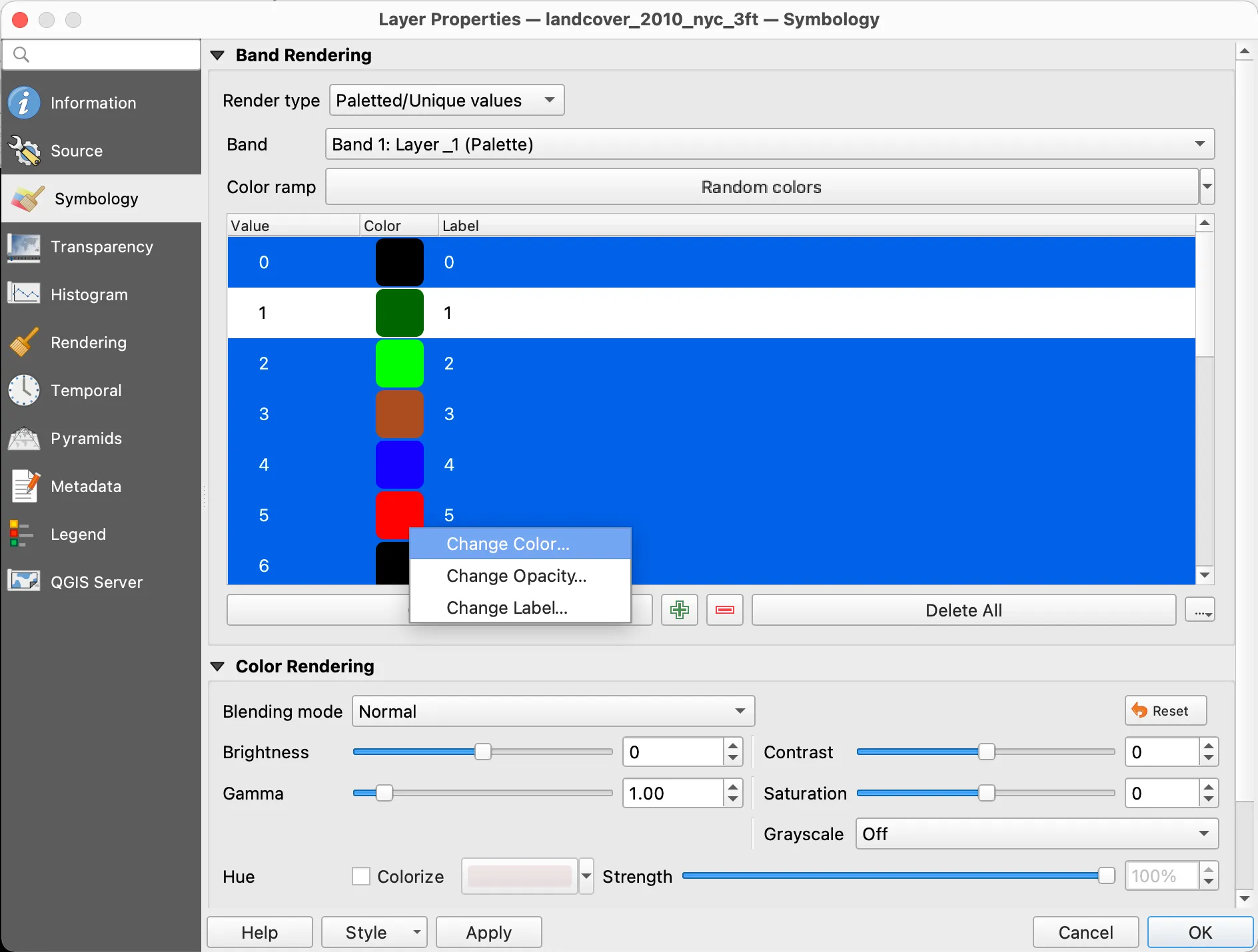Layer Symbology menu in the Layer Properties panel for NYC Land Cover

Change them all to white. Click OK on the change color menu then click Apply on the layer properties symbology menu. You should now see a map showing just those areas classified as tree canopy in this land cover dataset. Click OK to close the layer properties menu.

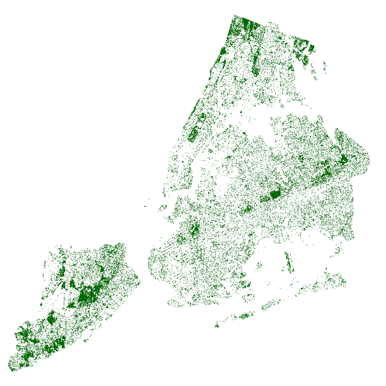A map of tree canopy based on land cover data

Adding vector data: creating points from XY values

To reduce processing times you will conduct the next section with a subset of data covering part of upper Manhattan (from 105th Street to 141st Street) which you downloaded in the data downloads section above. If you have a powerful computer (or don’t mind waiting several minutes between steps) feel free to download the complete version of the dataset for NYC as a whole.

• Download NYC Street Tree Census for all of NYC. Metadata available here.

We will add the results of the 2015 Street Tree Census to the map. This dataset is made available in tabular form (as Comma Separated Values) with coordinates specifying the location of each tree stored as columns in the dataset. QGIS can read these values and create a new vector dataset of points representing their locations.

From the top menu bar select Layer and then Add Layer > Add Delimited Text Layer.

When the Data Source Manager menu appears click on the ... and navigate to the data folder for this assignment. Select the 2015_Street_Tree_Census.csv file. Take a look at the preview of the dataset that appears at the bottom of the window. This allows you to see the columns included in the dataset as well as sample values. Scroll to the right to take a look at the available columns of information about each tree. You’ll notice that there are columns at the far right that specify the latitude and longitude coordinates for each tree. We will use these to create our new vector dataset specifying the point location of each tree.

Select the fields (columns) from the dataset that should be used to generate the X (longitude) and Y (latitude) coordinates for each point, QGIS may have already pre selected them for you.

Then make sure to specify the Geometry CRS as World Geodetic System (WGS) 84 (which has EPSG code 4326). This tells QGIS which coordinate reference system your point coordinates are defined in. We didn’t have any information with this dataset about the specific coordinate reference system used, however we can be confident of our choice of WGS 84 because (1) latitude and longitude coordinates always refer to a geographic coordinate reference system (they are angular units) and (2) the Global Positions System (GPS) which was most certainly used to generate these point locations uses WGS 84. We will cover coordinate reference systems and projections in week 3 but feel free to review this article from the Smorgasbord for an introduction to coordinate reference systems.

Click Add. It may take a few seconds to render the street tree locations.

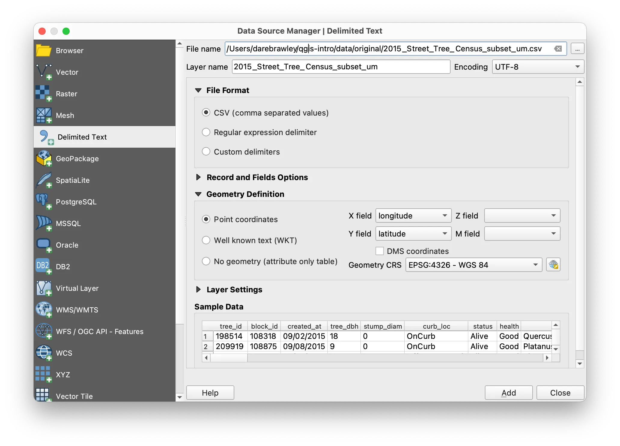Data Source Manager to add delimited text

Turn off the blocks and land cover datasets in the layers panel (uncheck the box next to the name of each) so that only the street tree locations are visible. Zoom in until you see an area that is a few blocks wide so that the individual trees are more visible.

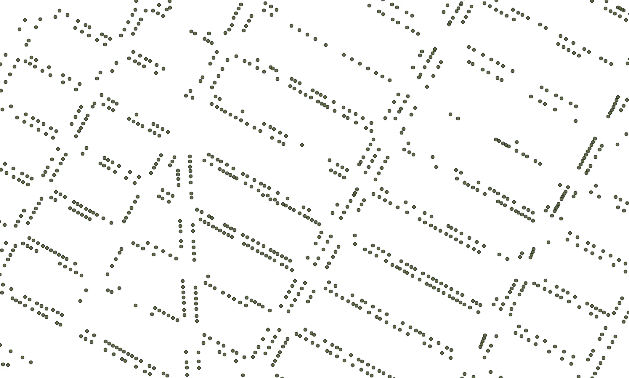Street trees visualized as points

Notice how the outlines of streets are visible in the patterns formed by the trees. It is also clear that some blocks have many trees and others have very few.

Because we created the street tree dataset from latitude and longitude coordinates, the dataset is not yet in the correct projected coordinate reference system for New York City. Like you did for the land cover data above, confirm the current coordinate reference system by right clicking on the street trees layer in the layers panel to open the Layer Properties menu. What is the current coordinate reference system (or CRS) for the street trees?

Because it is not yet in the New York State Plane-Long Island coordinate reference system we need to re-project the data.

To do this we will export a copy of the dataset and specify the new projected coordinate reference system that we wish to use.

Again right click on the street trees layer in the layers panel. Select Export>Save features as then in the Save vector features as dialogue window opens use the ... button to choose a location to save the new dataset you are creating (within the data>original folder you created for this project is a good spot). Specify the correct coordinate reference system for NYC (New York State Plane - Long Island with EPSG:2263). If it is not visible in the drop down menu click the Select CRS button to open the coordinate reference system dialog box and search for the correct coordinate reference system for NYC. Make sure Add saved file to map is selected and click OK. It may take a few minutes for this action to finish processing (there are a lot of street trees!).

Save vector layer dialogue box

Once the new dataset of street trees in the correct projected coordinate reference system you can remove the original street trees dataset from your project. Right click on its name in the Layers Panel and select remove layer.

Quantitative symbology: graduated symbols

Next we’ll make a map of trunk diameter by tree.

Open the layer properties menu and the symbology tab for the 2015_Street_Tree_Census_subset_um layer. Choose graduated symbols and then make the following selections:

Graduated symbols via the Layer Properties panel

Your map should look something like this:

A map of street trees visualized in two ways

Print Layouts in QGIS

From left: International Map of the World, Hudson River, 1927, US Geological Survey; Maps by Studio Joost Grootens from Atlas of the New Dutch Water Defense Line by Clemens Steenbergen et al, 2009; Passonneau & Wurman, “Cleveland” in Urban Atlas: 20 American Cities, 1966.

This section covers the basics of creating a print layout in QGIS and some considerations for cartographic design in general. The technical material covered allows you to move your QGIS projects from map space to paper space and to export your work either in a final presentation format or in a form that allows you to continue design work in another software environment.

Map space / paper space

So far you have worked within QGIS’s map canvas viewing and analyzing datasets. This environment gives a view of your data from whatever spatial scale you set through the zoom and pan setting in the map canvas view. We can refer to this environment as map space. In order to export your work from QGIS so that it can be viewed as a static image outside of the program you must fix the spatial scale of your work. Like work in CAD softwares this can be understood as paper space. The Print Layout function within QGIS is a tool that enables this transition into paper space.

Cartographic design

The transition from map space to paper space also affords you the opportunity to begin to think about aspects of cartographic design that are not relevant when performing analysis in QGIS.

How will you orient readers of your map to the geographic context of your map? How will you convey the meaning(s) of the symbols you have chosen?

Maps typically have:

• a legend
• an indication of scale (either a scale bar or in the case of printed maps a written scale 1”=1000 feet for example)
• a note showing the projection used
• a north arrow
• citations for all data sources
• the name of cartographer and/or publisher
• (sometimes) a grid and/or a graticule to convey the coordinate reference system

The examples shown at the opening of this tutorial highlight some examples of the above listed map elements.

Set up

In the main toolbar of your QGIS project select the New Print Layout tool, or select Project>New Print Layout from the top menu. You will be prompted to specify a name for your new layout. Each QGIS project can have multiple associated print layouts so choose a descriptive name for the layout you are hoping to create so that you can distinguish it if you ever add an additional layout view.

Once you have specified the name of your first layout the print layout tool will open.

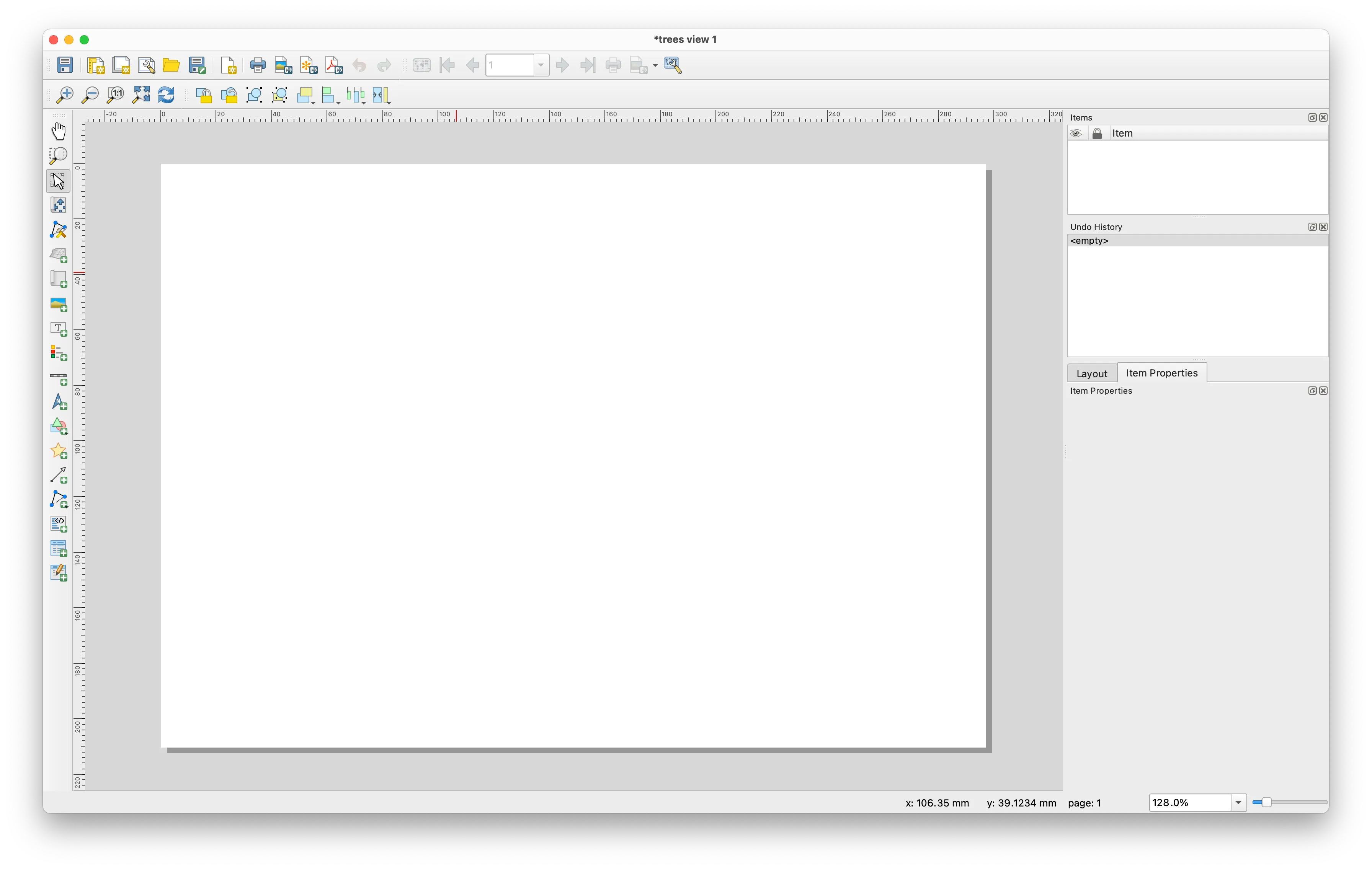
Set page size

To set the page size right click anywhere on the blank page and select Page Properties. The Item Properties menu should appear. Use this to specify the dimensions of the page. There are preset paper sizes and you may also specify your own size using the Custom option and choosing specific dimensions and units.

Add a map

Use the Add Map button and then click to draw a rectangle over the area on your page that you want the map to cover.

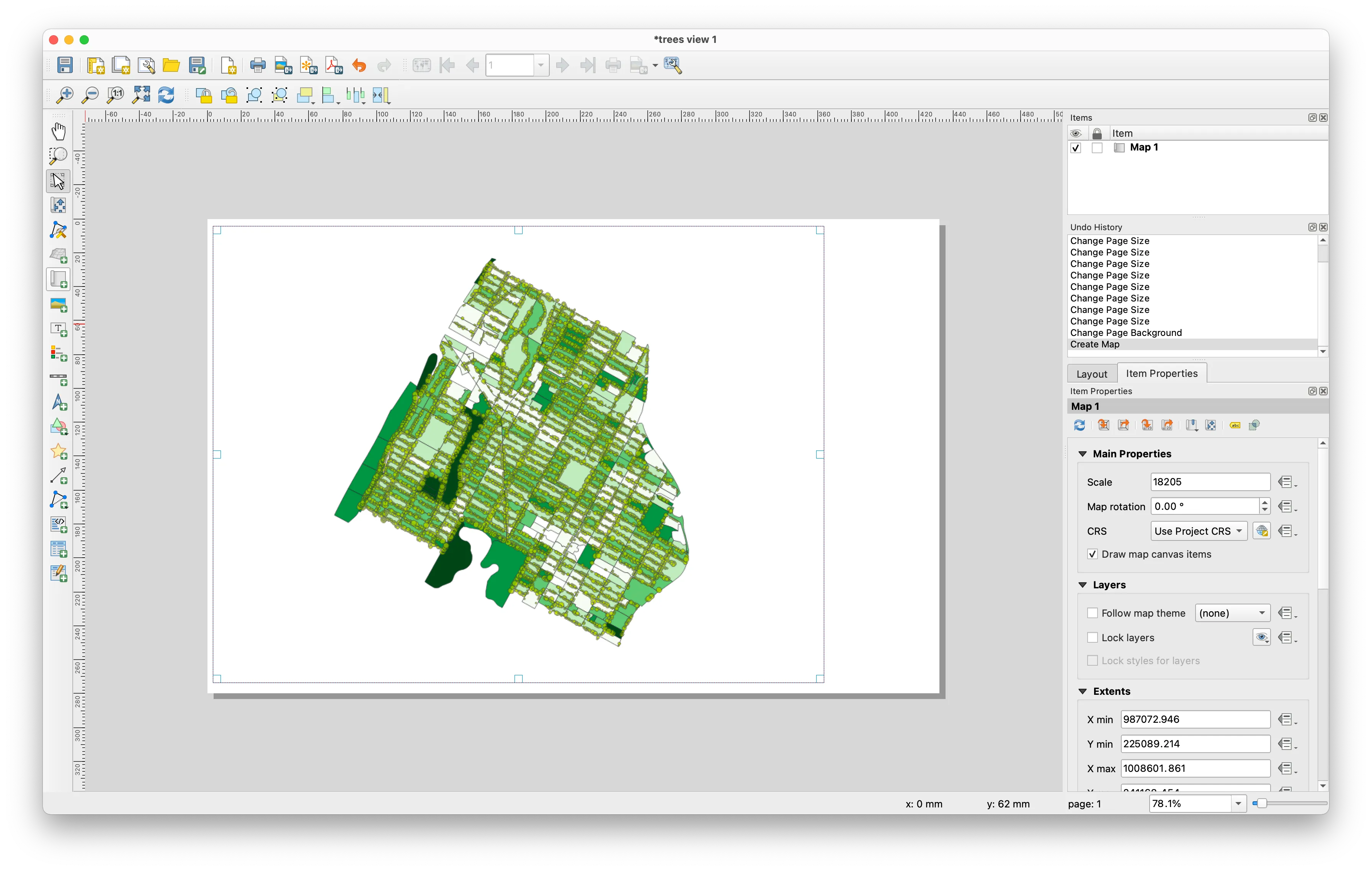
Edit item properties

In general, to adjust styling or properties for each map element within the print layout tool select the element on the map and then open the Item Properties tab. The Item Properties menu provides styling and other options specific for each map element.

For a map element you can adjust the scale, the coordinate reference system(CRS) that the data is viewed in, the rotation of the map, which layers are visible, the spatial extents of the map view (specified in coordinates of the CRS of your map project) among other options.

Set your preferred map scale & experiment with the map rotation. Setting the map rotation at -28.7° when using the New York State Plane Long Island projected coordinate reference system will align the Manhattan street grid with the page.

Add a legend

Select the Add Legend button and again draw a rectangle over the area where you want your legend to be placed.

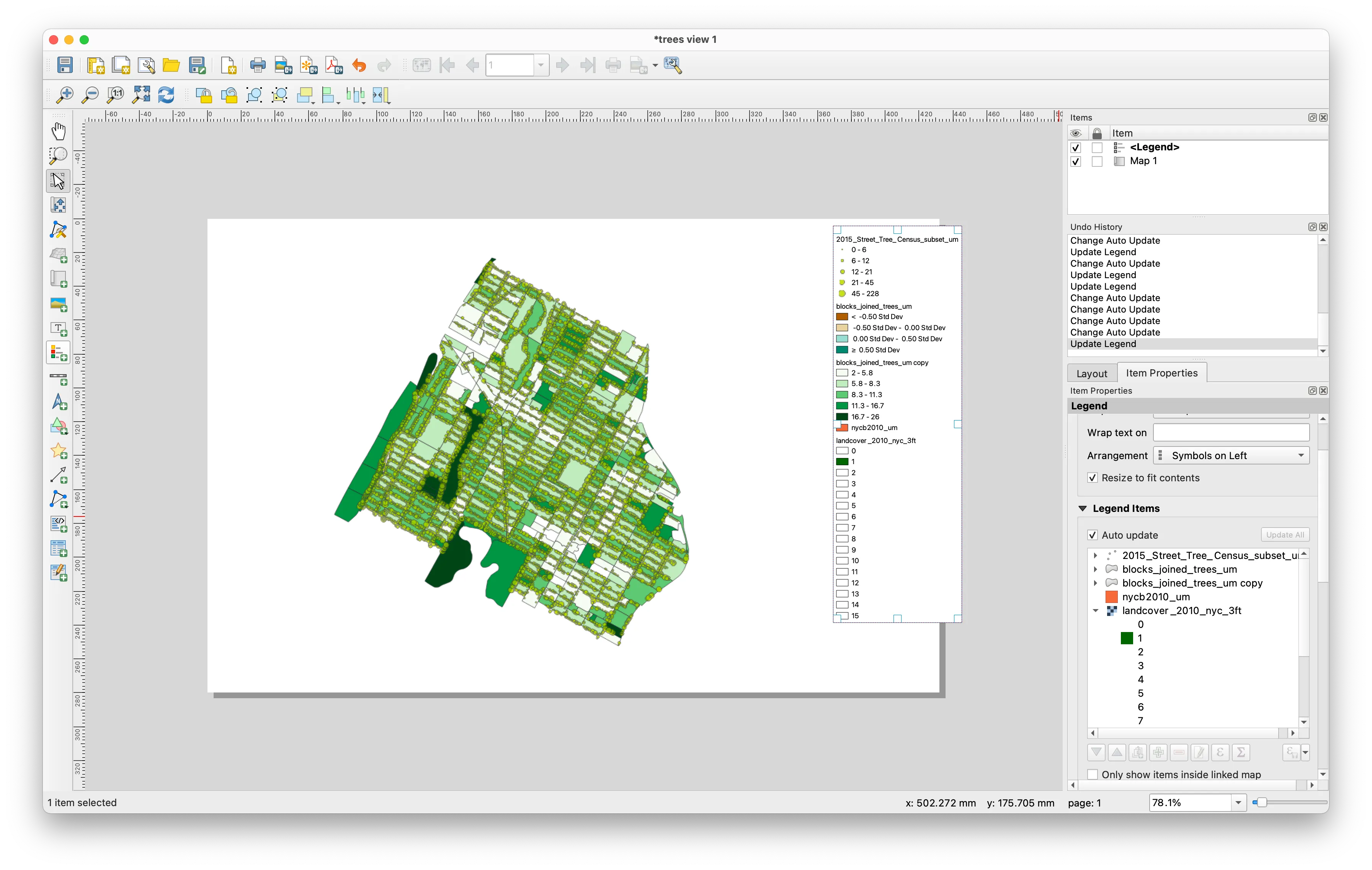
By default all layers from your QGIS project will be included in the legend. If, within the Item Properties for your legend, you select Only show items inside linked map then only the currently visible map layers will be included in the legend. If you would like to manually select which elements to include in the legend then deselect Auto Update. You can then use the + and - buttons to add and remove legend elements.

Add a grid

A grid can help to convey the location of a map within a given coordinate reference system. A map grid displays vertical and horizontal lines at defined intervals of given coordinate reference system. A graticule refers specifically to the display of geographic coordinates (degrees of latitude and longitude).

A map can have multiple grids and/or a graticule to convey the location of the map across multiple coordinate reference systems.

Add a grid for the coordinate reference system of our map (New York State Plane Long Island NAD 1983) as well as a graticule.

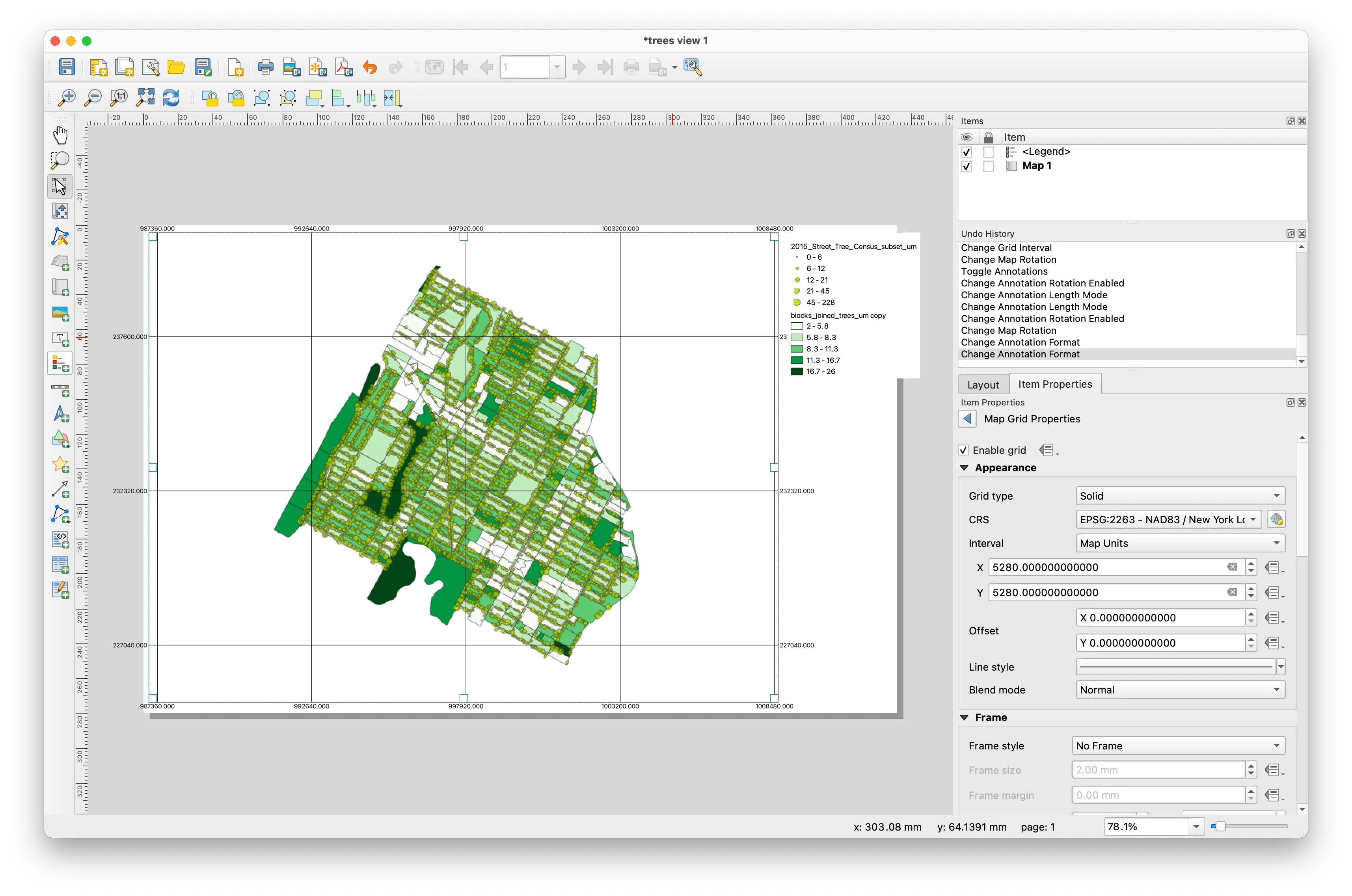
Select the map and view its item properties. Scroll to and expand the Grids section. Use the green + to add a new grid. Name the grid EPSG 2263 (the CRS of the map).

Select modify the grid. And make the following selections: for CRS EPSG: 2263; interval map unit; x 5280 y 5280 (aka 1 mile). Scroll down to Draw coordinates. Select the check box. For format select decimal. You can also adjust the size, placement, and font of these coordinates within this item properties menu. Once you are pleased with their appearance, leave the grid item properties menu with the blue arrow at the top of the item properties menu.

The map now displays a grid showing the coordinate reference system.

Next create a graticule to overlay on the map. Create a new grid as before. Name it WGS84 (this is a geographic coordinate reference system). Select modify grid make the following selections: CRS EPSG: 4326; interval map unit; x & y as 0.03/

So that you can distinguish with the other grid change the color or stroke style by selecting the Line dropdown menu. Scroll to enable Draw Coordinates. Format as degree, minute. Change the font color to match the color you chose for the lines

Note: Grid enabled at the top of the grid properties menu toggles visibility for the grid.

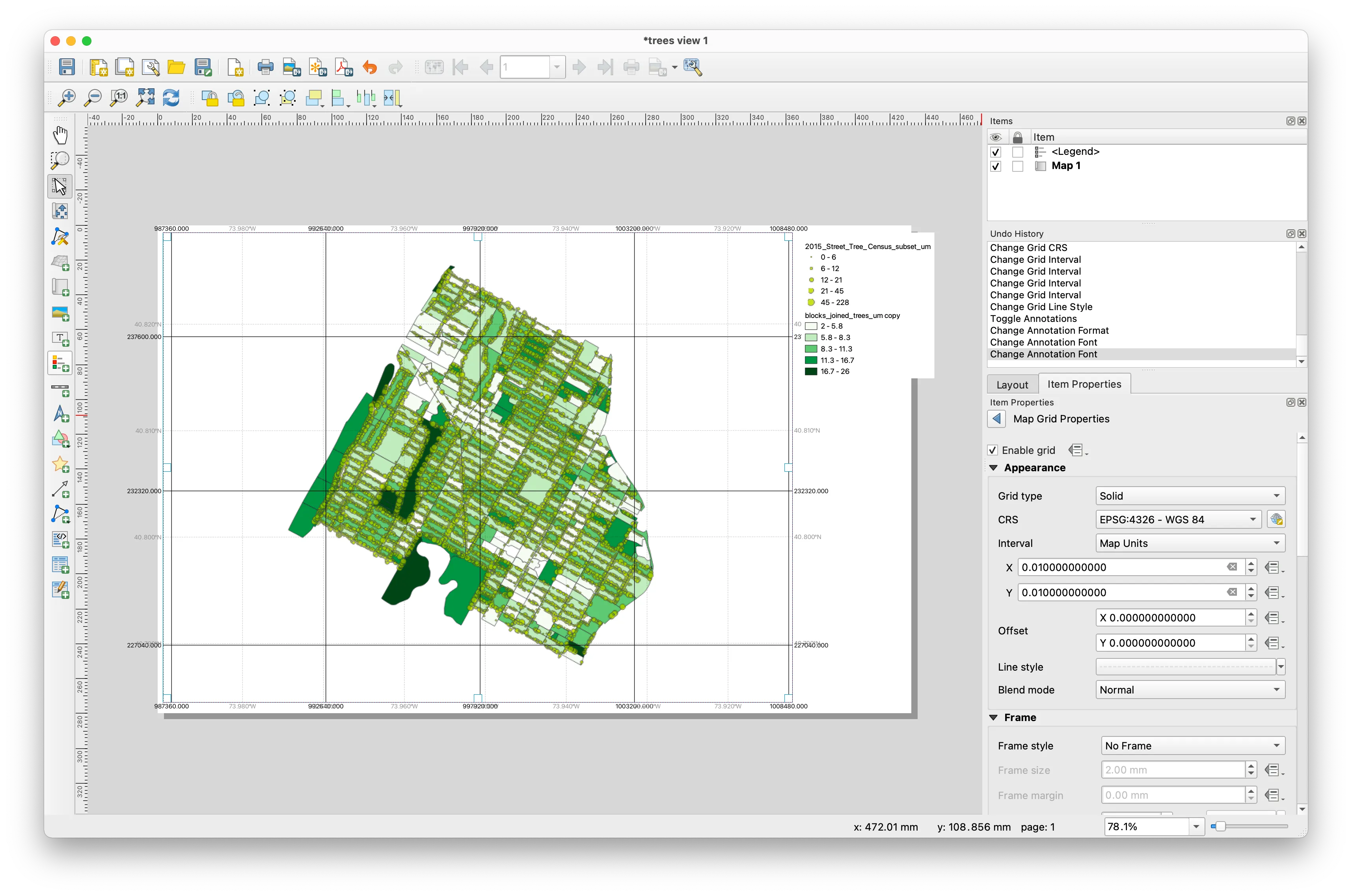
Notice difference between the grid and the graticule. Based on the projections and coordinate reference systems module can you interpret these differences?

Add additional map elements

Use the left toolbar to add a north arrow and a scale bar. Adjust the style and settings for each using the Item Properties menu for each element.

Exporting

It is possible to export a print layout in multiple formats including as a PDF, as an image file (in multiple formats), or in SVG format.

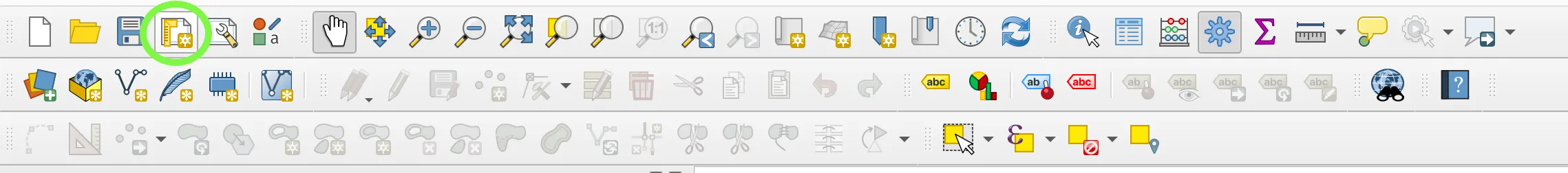
Export options can be accessed via Layout in the top menu bar or the export buttons in the Layout toolbar (circled below).

Notes on workflow

It is possible to use the print layout tool within QGIS to design visually compelling maps. However, it is generally much faster to use the print layout to: define a map/paper size, set the spatial scale of your map(s), and add any orienting map elements (scale, legend) and then export to continue your work in a dedicated graphics editing software.

Exporting maps with vector-based data in SVG format allows you to edit the representation of your data in Illustrator or another vector graphics software.

Any raster-based data should be exported separately as in a high resolution image format which can be layered in your graphics editor of choice with any vector-based elements.

Deliverables

One map of trees in NYC composed as a 8.5x11 page (landscape or portrait orientation) exported as a PDF. Your map must include standard map elements outlined above. Please submit via Canvas in advance of class on 9/13.

Further resources

Print-layout how-to:

• The QGIS documentation has a detailed overview to the Print Layout tool, available via the docs here

Map design more generally:

• Mark Monmonier’s How to Lie with Maps is a classic now in its 3rd edition on concerns and approaches for cartography and cartographic design.
• In cartography (as with all design work) being able to produce thoughtful projects begins by developing visual literacies and fluency with cartographic conventions and how to subvert or extend them. The best way to approach this is to look at many many precedent projects. Historical and/or maps designed for print are often a good starting point as they tend to be more thoughtful in their use of cartographic elements than maps designed for the web. David Rumsey Map Collection is a good source for archival maps with global coverage. Spend time with atlases and search for cartographers whose visual style you like.