World Projections and Coordinate Systems

As the world is a 3D object, it is impossible to represent it in 2D without some distortion. This is the problem of projections. Projections are the mathematical formulas that transform the Earth’s 3D surface into a 2D plane. Thankfully, GIS software can be used to perform these transformations in near real time. Because of this, we may take for granted how space is distorted based on which projection is chosen.

In the exercise, you will explore how projections impact our conception of distance by moving between GIS and CAD software. You could explore these same concepts using Python instead of either. Specifically, you will:

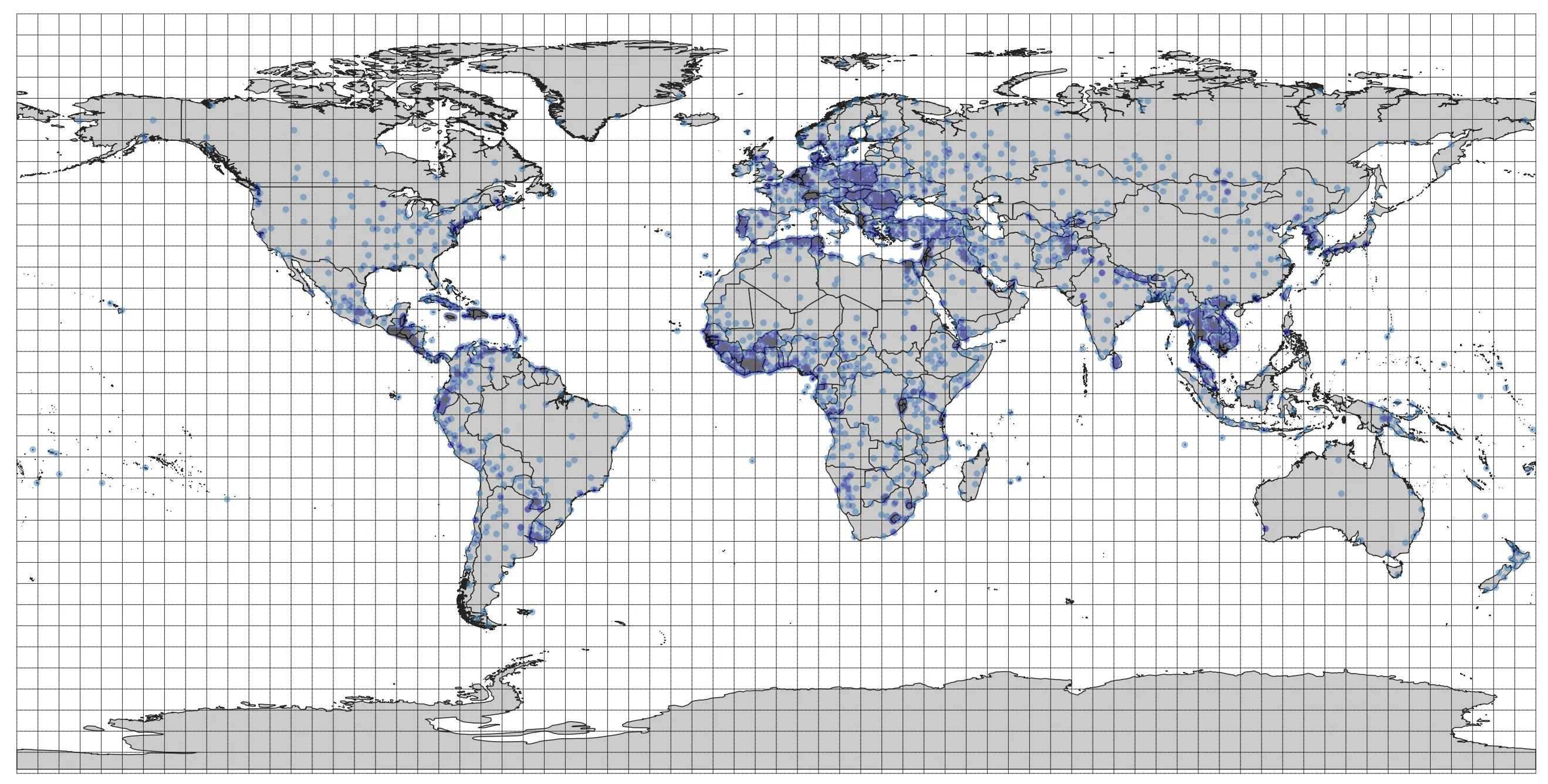
• Create a new map with country boundaries, points representing world cities, and a global grid
• Change the map projection so that all layers are represented in an Equidistance Conic projection
• Reproject and save new copies of files so that all files are in the same projection
• Import these layers into Rhino using Grasshopper
• Calculate the shortest paths between multiple cities
• Import these paths back into your map
• Visualize the shortest paths in a number of different projections
• Compose map visualizations to submit

Deliverables

Four maps, composed as landscape 8.5x11 pages and submitted as a combined PDF. Each map should clearly depict the lines that extend between cities, the distances between each, and a representation of the cities themselves. Remember that the primary goal of each map is to convey the spatial relationship between the cities you chose, so the map scale and layout should reflect those relationships appropriately.

Data

• World Cities are available from Esri’s ArcGIS Hub
• World Countries are available from Esri’s ArcGIS Hub
• World Lat/lon grid

Exercise

Getting Started

Create a new project, either in QGIS or a Jupyter notebook. Add the world cities and world countries layers to your map. Represent each layer such that you can see the distribution of cities across the continents. Use the attribute filter to only show five-degree intervals to improve legibility, and add the grid as the top drawing layer. Adjust line weight and the colors in your map to maximize legibility.

Inspecting projections

Each of these different datasets has an idea of its coordinate reference system- it knows where it’s origin is, what datum it refers to, and what projection it is in. In desktop GIS software, that is why map layers are able to reproject “on the fly”- the software knows how to apply conversions so that the spatial relationship between layers is what we expect. Mapping with GeoPandas is less automatic- if we plot two layers with different coordinate systems together on the same plot, they may appear very far away from each other.

Open the world countries layer properties and observe what coordinate system it uses. If you are using QGIS, confirm that the project’s coordinate system matches this layer’s coordinate system. If you are using Python, make note of this projection, as it is what we will use moving forward. In both cases, we will end up re-projecting layers into this coordinate system.

• To check a layer’s CRS in QGIS, right click on a layer > Properties > Information (or double click on the layer > Information) and verify the information
• In Python, print the layer’s crs property: layer_name.crs
• If the layer in question is a shapefile, you can open the .prj file. If you are working with a .geojson file, the crs information will be at the top of the file.

Changing the map document’s projection

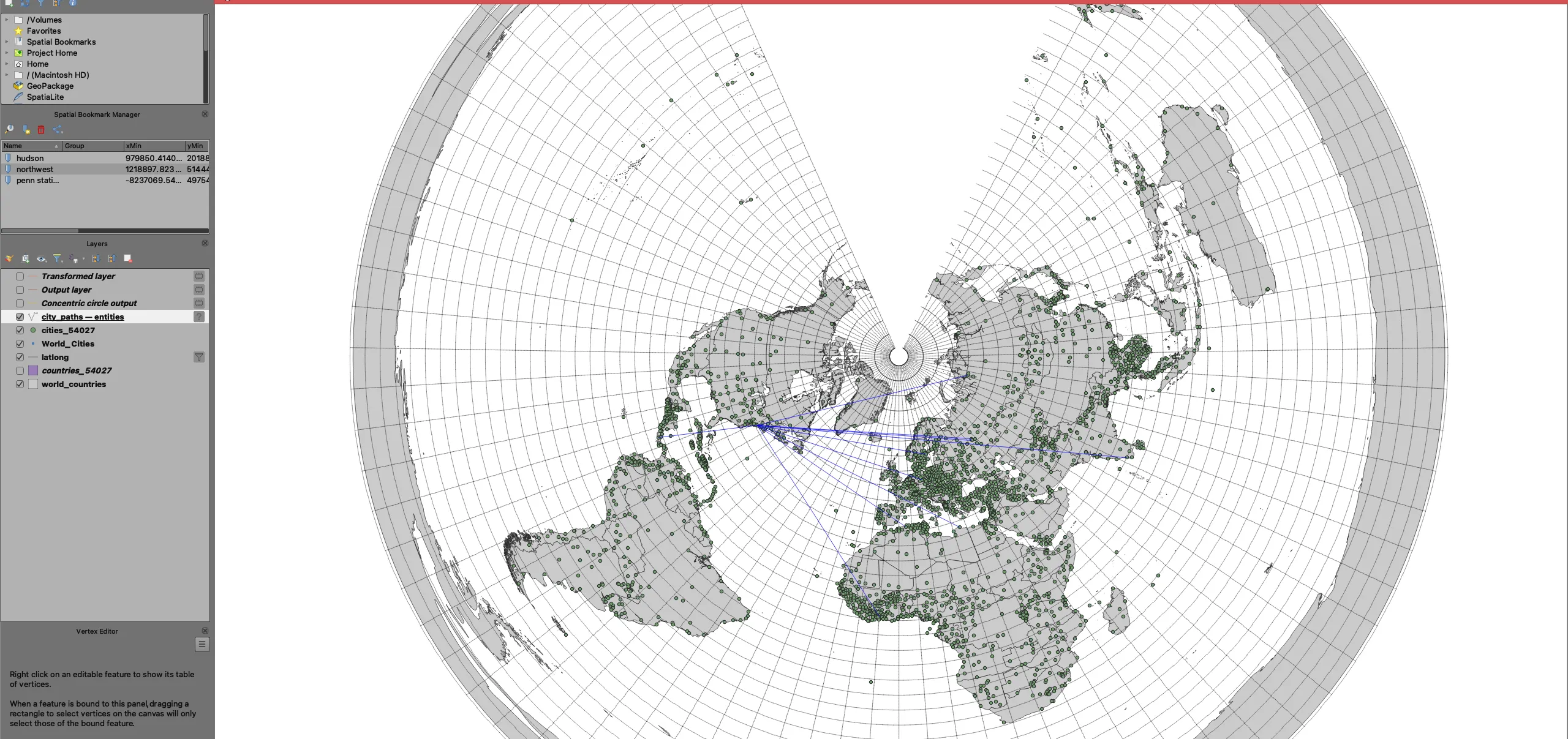
We will utilize a projection developed by ESRI to view the world in an equidistant, conic projection. This means that the distances between points on the world are preferenced over the size or shape of points on the earth. Information about this projection can be found here. In the lower right hand corner of your QGIS window, click on the Current CRS selector, which launches a CRS selector wizard. In the search bar, type 54027 and then select the result.

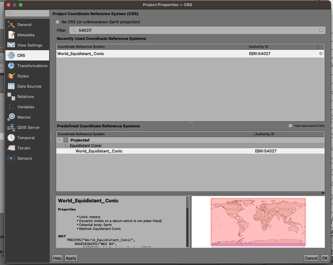
Now when you click OK, you will see the world under this other projection system.

Changing projections

Remember, without changing the projection of the file, layers will look correct per a given projection, but are still internally in reference to the coordinate system of the file. We must reproject the layer to the target projection system to be able to perform analysis or use the layer in another software. Note that this is different than “changing” the layer’s projection system- changing the system without reprojection will set a different origin without recalculating new feature geometries.

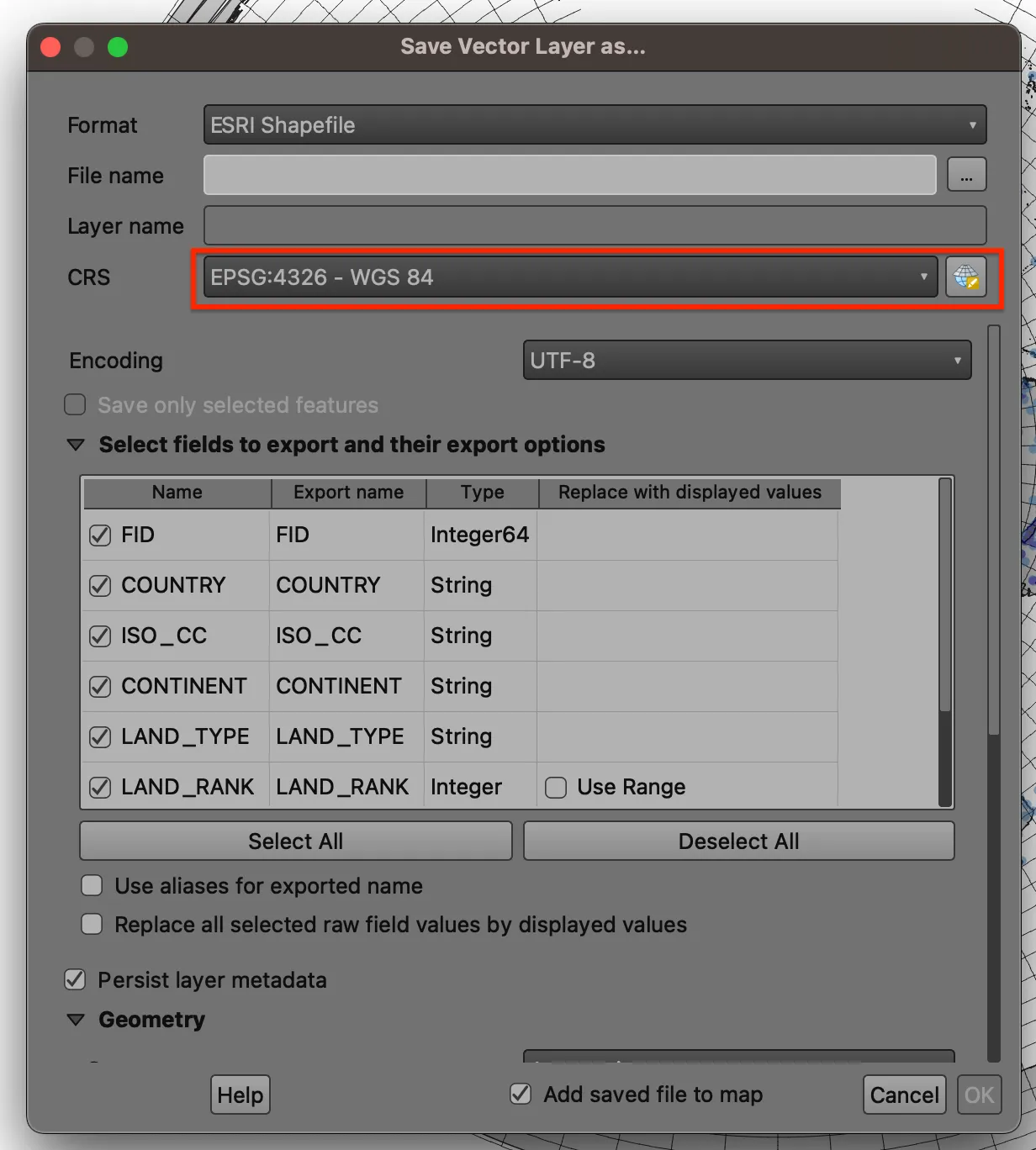
To reproject the layer in QGIS, right click on the layer in the layer tree, and click Export > Save Features As....

Click the ellipsis to save your file in your project folder. By default, QGIS will attempt to save files in your computer’s root folder. Then, use the CRS dropdown to select 54027, the projection we are using for this exercise. This will ensure that the layer, and not just how the layer is represented in the QGIS session, reflects this projection system.

Export both the countries and cities layers in this new projection.

Drawing shortest paths between world cities

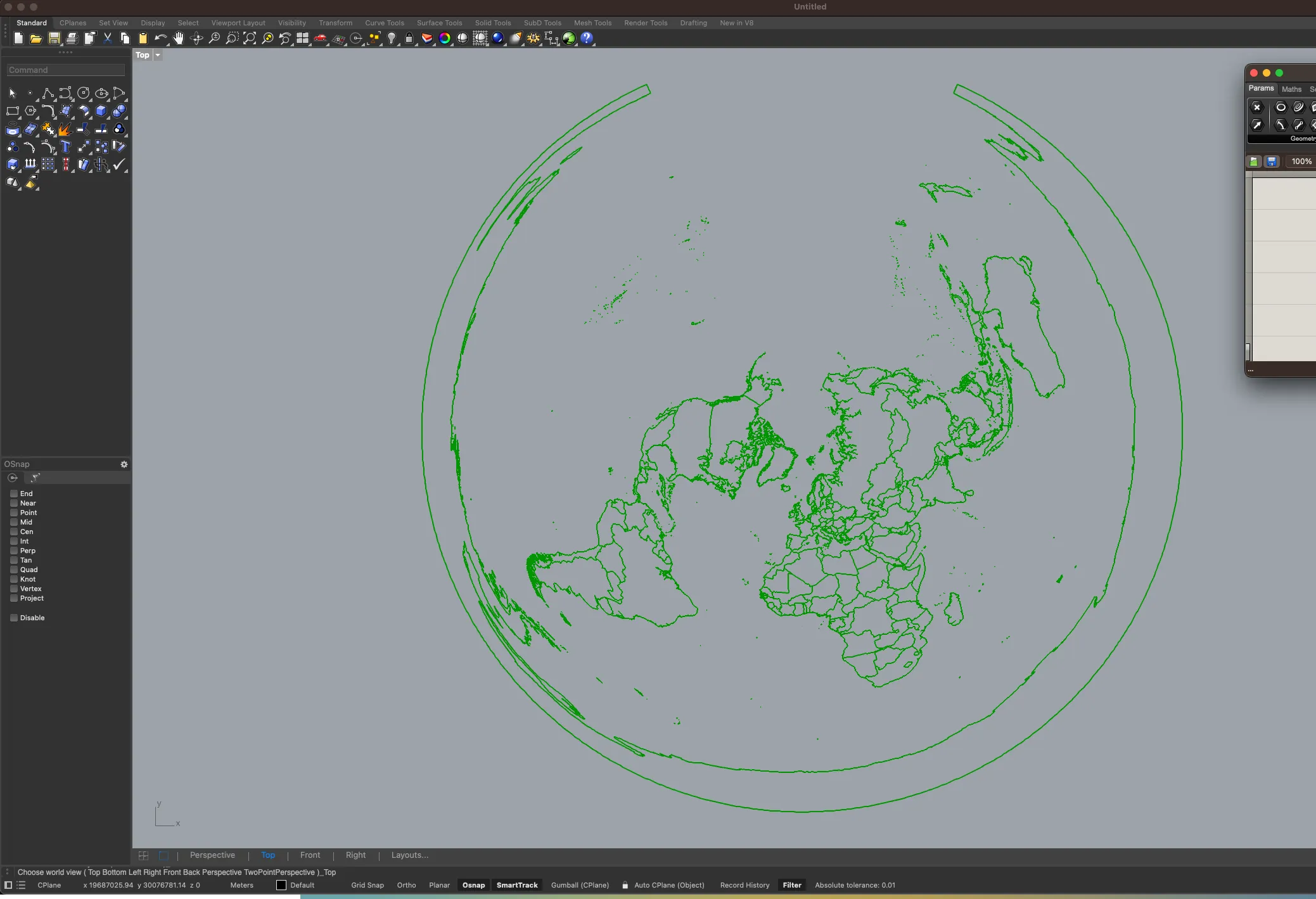
Open Rhino and create a new project for large objects in meters. Launch Grasshopper. In a new canvas, search for the Import SHP component and attach a File Path component. Right click on the file path component and click on Select one existing file. Navigate to your newly created shapefile and select the file ending with .shp. Select the Import SHP component, and then right click on the canvas to select Zoom- this will recenter the Rhino window to the component’s solution. You will now see the world in the projection we selected.

Note the x and y coordinates in the bottom left corner of the Rhino window- we see that as we move our cursor across the canvas, the position is reported back to us in meters, matching the coordinates we saw in QGIS. In Grasshopper, right click on the Import SHP component and bake the solution to a layer. Now we will be able to interact with the geometry in Rhino.

Perform the same process with the world cities, baking the points to a different layer. We are now ready to draw shortest paths between world cities.

There are a few options for selecting cities for this exercise, but the final goal is to draw shortest path lines between cities a handful of cities.

Some options include:

• using the Line or Curve command in Rhino to draw a series of straight lines between city points
• using Grasshopper to identify a city and then selecting a series of cities (randomly or otherwise) to draw lines between

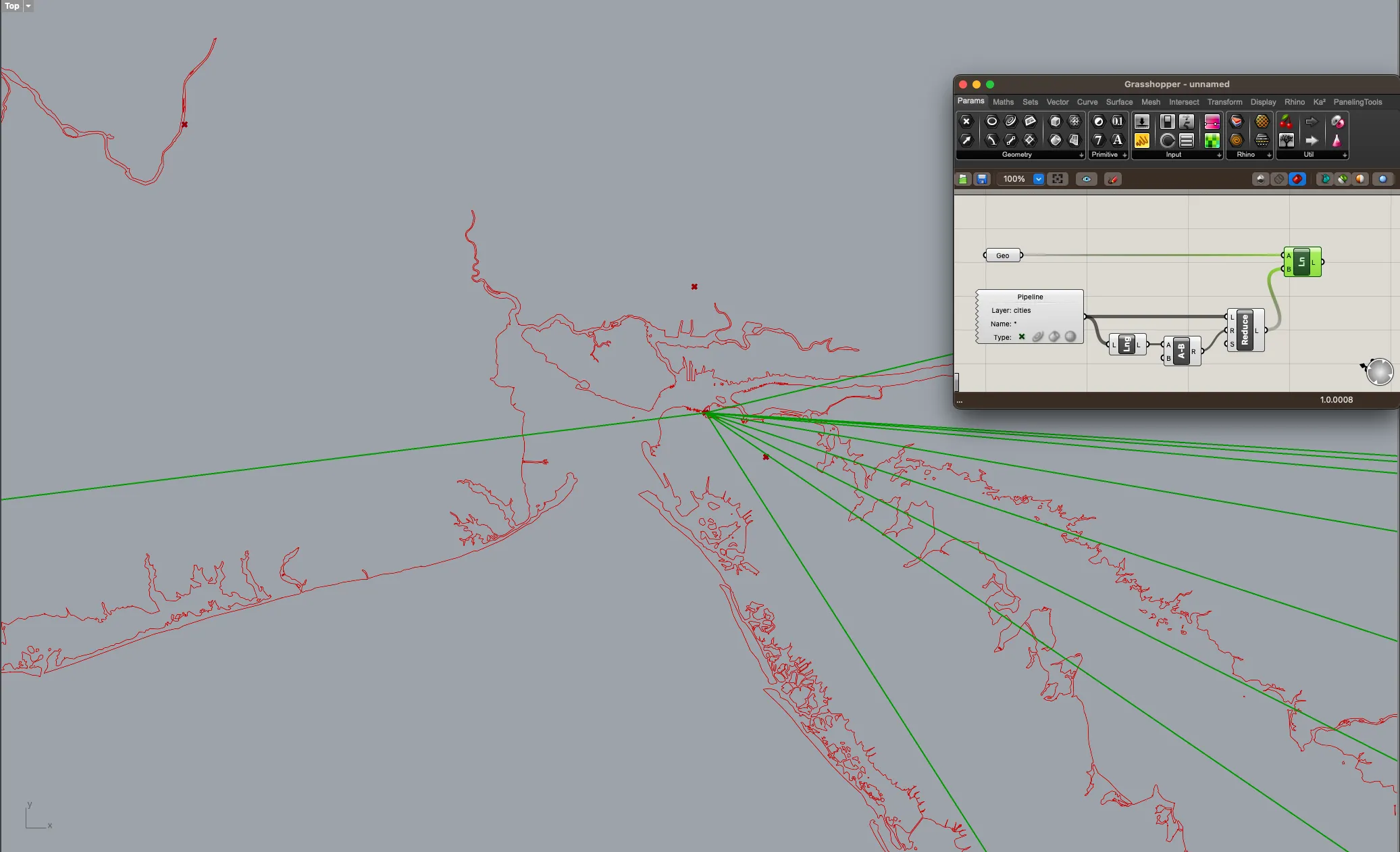
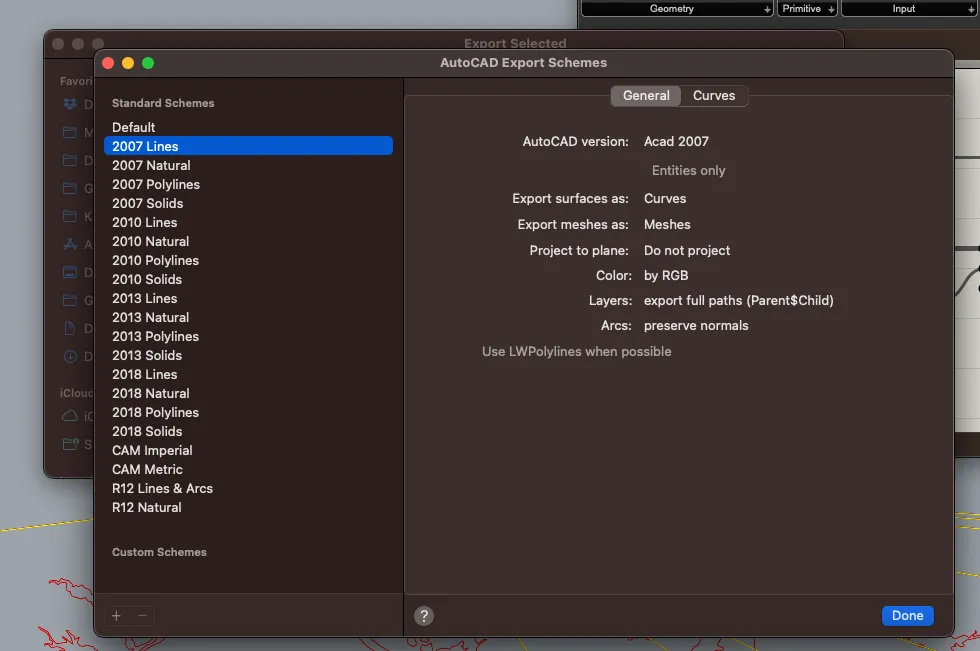
Regardless of how you create your lines, once you have finished, select the geometries and in Rhino navigate to File>Export Selected. Save the file in the .dxf format to your project folder using the 2007 - Lines option in the Edit Schemes interface.

Importing into QGIS

Return to your QGIS window. Add the newly created layer to QGIS. As you add the layer, you will notice that it does not inherently know what CRS to use, yet it should register properly on your map. You can set the projection by clicking on the question mark next to the layer name in the layer tree. Set the CRS to 54027. Save the file as a shapefile for use in the next step.

Inspecting results

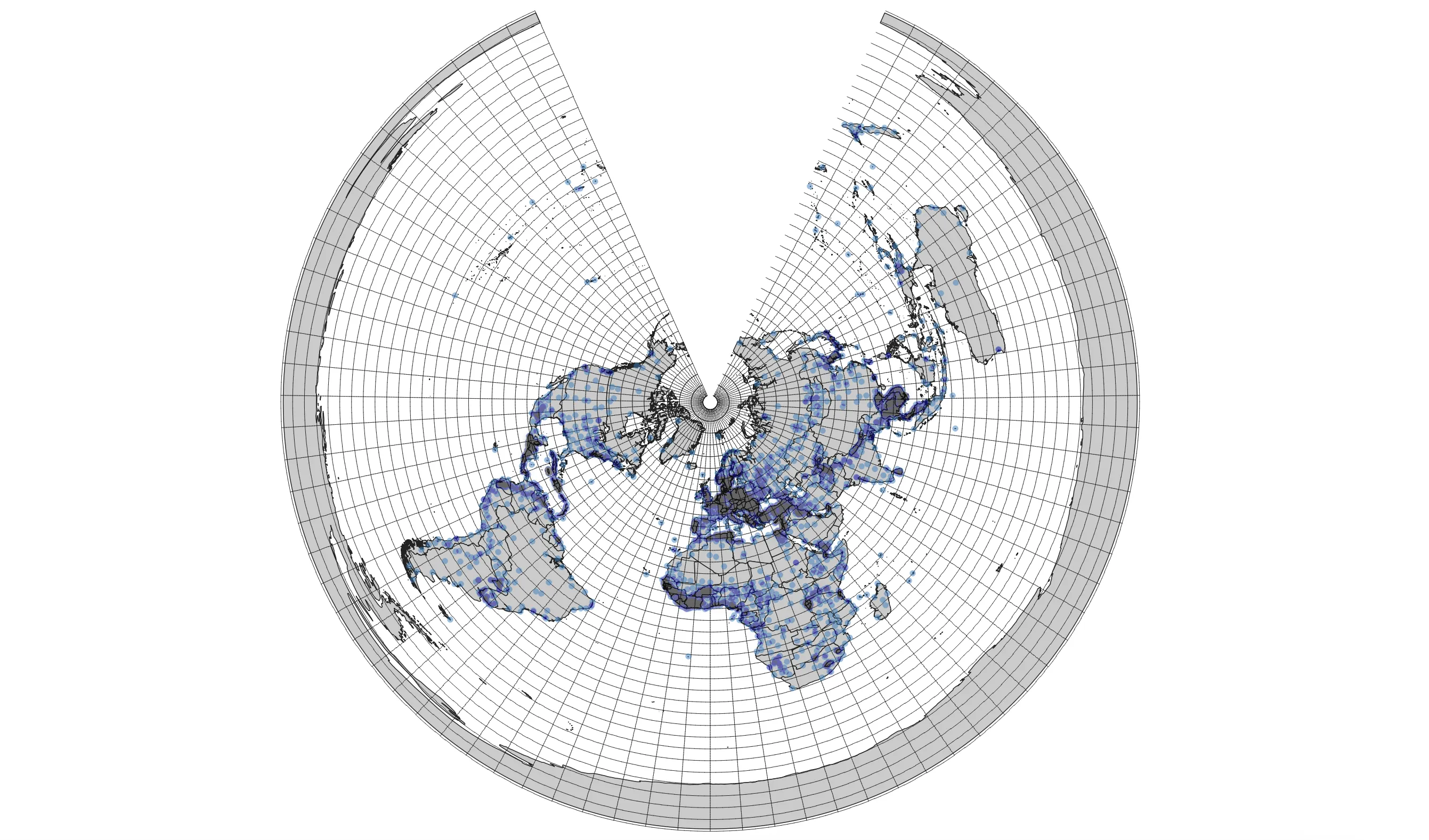
Change the map project projection to 4326. We will use the Shape Tools plugin to visualize the results in other coordinate systems. Click on Plugins>Manage and Install Plugins... and search for Shape Tools. Install the package. Once the package has been installed, go to Vector>Shape Tools>Geodesic Shape Densifier.... Select the shapefile you created in the previous step and set an output location.

Once the tool finishes, you will see the shortest path lines expressed relative to the curvature of the earth.

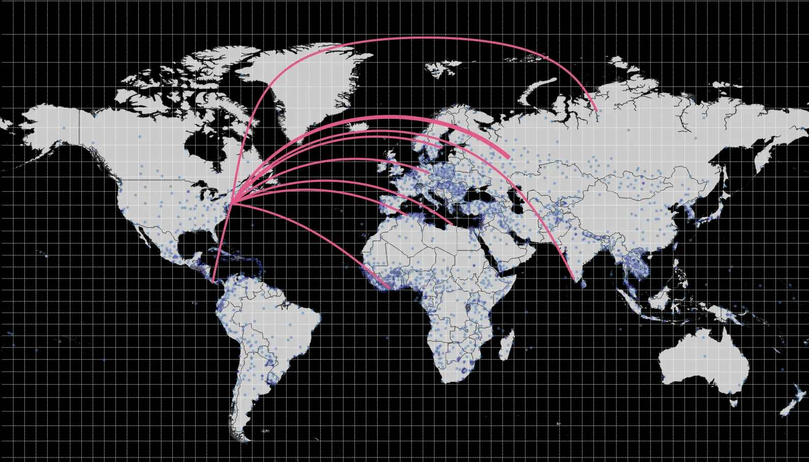
Note the differences compared to the straight lines that you drew in Rhino.

Per the deliverables listed above, you must submit four PDF maps that clearly represent these lines, and the cities they connect, to a lay audience. Choose three projections that represent the world at the global scale (filter by typing “world” in the Project Properties - CRS menu). Some examples include World Gall Stereographic and Robinson \